Individual dataset processing

Author

Ricardo Martins-Ferreira

Example for the Grubman et al. 2019 dataset (PMID:31768052)

The following script was applied to the Grubman dataset, which consists of single-nucleus (sn)RNA-seq in postmortem entorhinal cortex from six healthy controls and six patients with Alzheimer’s Disease (AD).

The data was accessed as a preprocessed count matrix and a covariare matrix, both available at GEO (GSE138852).

Load required packages

libs <- c("Seurat", "tidyverse", "stringr", "data.table", "readxl")
suppressMessages(
suppressWarnings(sapply(libs, require, character.only =TRUE))
)

    Seurat  tidyverse    stringr data.table     readxl 
      TRUE       TRUE       TRUE       TRUE       TRUE

Create Seurat object from count matrix

Upload the count matrix with 13,214 nuclei and 10,850 genes. Create Seurat object to include only genes present in at least 3 nuclei.

Seurat = CreateSeuratObject(counts =count.matrix, min.cells=3)

Filter low quality nuclei

Remove nuclei with the following features: - Feature counts lower than 200 and higher than 5000; - UMI counts lower than 500 and higher than 20000; - Percentage of mitochondrial genes higher than 20%: - Percentage of ribosomal genes higher than 5% (only applied to snRNA-seq data).

# Calculate the percentage of ribosomal genes
C<-GetAssayData(object = Seurat, slot = "counts")
rb.genes <- rownames(Seurat)[grep("^RP[SL]",rownames(Seurat))]
percent.ribo <- colSums(C[rb.genes,])/Matrix::colSums(C)*100
Seurat <- AddMetaData(Seurat, percent.ribo, col.name = "percent.ribo")

# Calculate thee percentage of mitochondrial genes
Seurat[["percent.mt"]] = PercentageFeatureSet(Seurat, pattern = "^MT-")

# Filter low quality nuclei
Seurat <- subset(Seurat, subset = nFeature_RNA > 200 & nFeature_RNA < 5000  & nCount_RNA > 500 & 
                    nCount_RNA < 20000 & percent.mt < 10 & percent.ribo < 5)

Seurat

An object of class Seurat 
10850 features across 11440 samples within 1 assay 
Active assay: RNA (10850 features, 0 variable features)
 1 layer present: counts

# check mean genes per nuclei
mean(Seurat@meta.data$nFeature_RNA)

[1] 756.6617

The used filtering pipeline originated a Seurat object with 11,440 nuclei, 10,850 genes and approximately 757 genes per nuclei.

Quality Control metrics

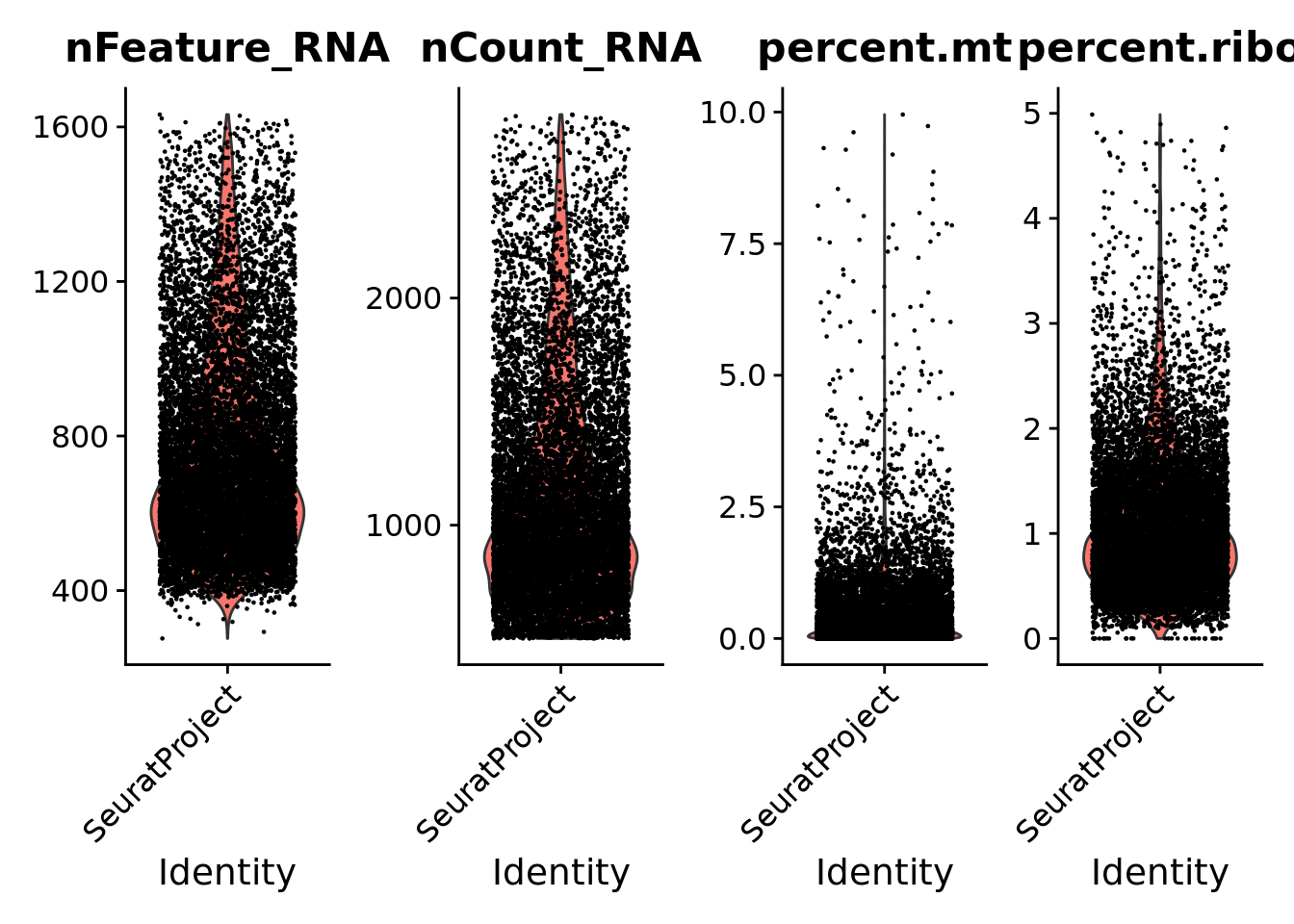
Visualize the number of genes and UMI counts per nuclei, and the percentage of mitochondrial and ribosomal genes as violin plots.

print(VlnPlot(Seurat, features = c("nFeature_RNA", "nCount_RNA",
"percent.mt","percent.ribo"), ncol = 4))

Warning: Default search for "data" layer in "RNA" assay yielded no results;
utilizing "counts" layer instead.

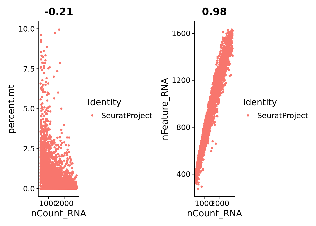
FeatureScatter representation of the association between the number of UMI counts per nuclei and the percentage of mitochondrial genes, and between UMI counts and the number of genes per nuclei.

plot1 = FeatureScatter(Seurat, feature1 = "nCount_RNA", feature2 = "percent.mt")
plot2 = FeatureScatter(Seurat, feature1 = "nCount_RNA", feature2 = "nFeature_RNA")
print(plot1 + plot2)

Annotate nuclei based on sample information

This dataset contains 3 controls and 3 patient samples, with each one being composed of two pooled individual samples.

Create a column in metadata (TAG) with the nuclei annotation.

Seurat@meta.data$TAG <- rownames(Seurat@meta.data)

The name of each sample (Sample_ID) is merged to each nuclei’s annotation. Split the sample name from the full nuclei name.

x<-as.data.frame(str_split_fixed(Seurat@meta.data$TAG,"_",2))
Seurat@meta.data$Sample_ID <- x$V2
head(Seurat@meta.data$Sample_ID)

[1] "AD5_AD6" "AD5_AD6" "AD5_AD6" "AD5_AD6" "AD5_AD6" "AD5_AD6"

Remove the columns on percent.ribo and percent.mt from the metadata.

Seurat@meta.data <- Seurat@meta.data[,-c(4,5)]

Filter out genes associated with postmortem interval

Remove the list of genes associated with postmortem interval in bulk RNA-seq in cerebral cortex (Zhu et. al 2017; PMID: 28710439). This list (“PMI-genes.csv”) is available on the “Support data” folder from this repository.

Note: In the original Grubman et al. study these genes had already been removed. This script was applied to all other datasets.

keep= c(!rownames(Seurat) %in% c(PMI_genes))
Seurat<- subset(x = Seurat,features =c(1:(dim(Seurat)[1]))[keep])

Seurat

An object of class Seurat 
10850 features across 11440 samples within 1 assay 
Active assay: RNA (10850 features, 0 variable features)
 1 layer present: counts

# check mean genes per nuclei
mean(Seurat@meta.data$nFeature_RNA)

[1] 756.6617

Doublet removal

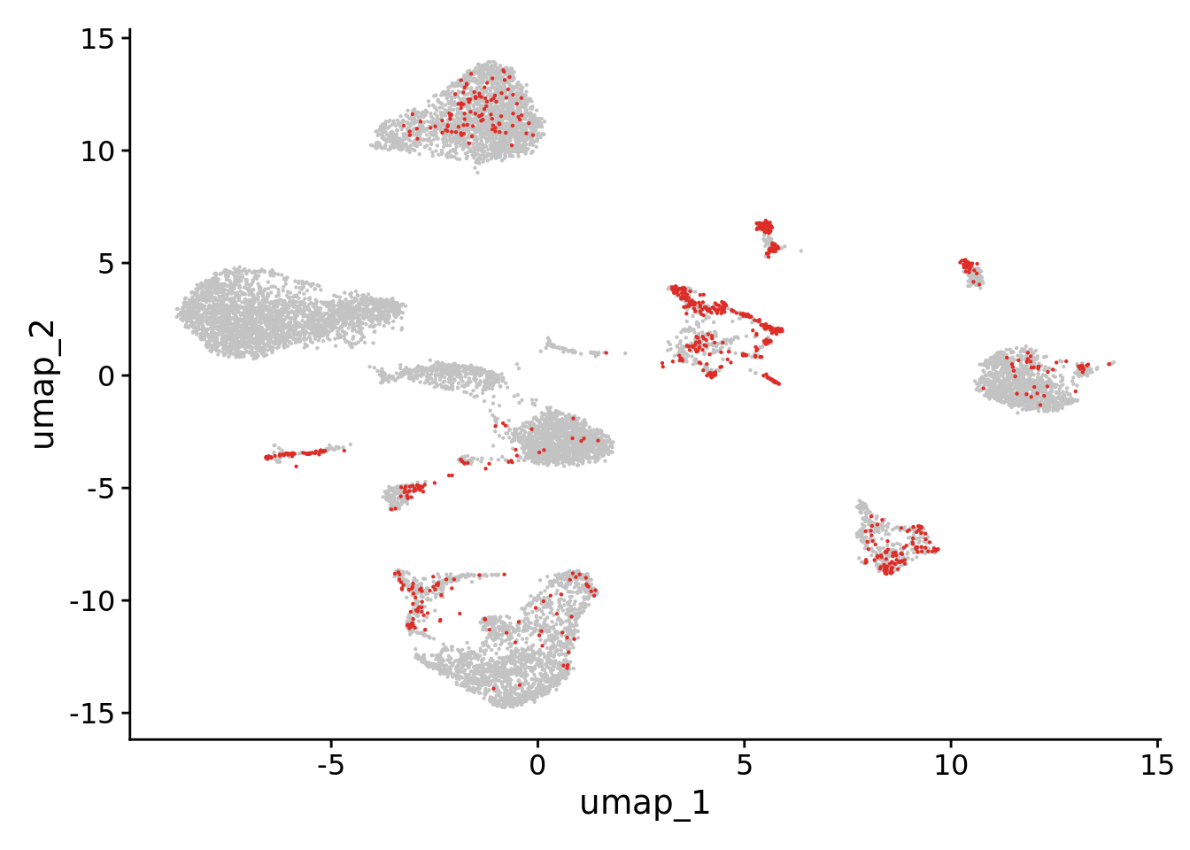
Doublets (n=858) had already been calculated using DoubletFinder (see script in “Double-Finder.html” in this repository). Upload a vector of nuclei (“doublets”) deemed as doublets. Plot the Seurat object highlighting the doublets.

Seurat <- SCTransform(Seurat, verbose = FALSE) #default variable features = 3000
Seurat <- RunPCA(Seurat, verbose = FALSE)
Seurat <- RunUMAP(Seurat, reduction = "pca",dims = 1:30, verbose = FALSE)

DimPlot(Seurat, reduction = "umap", cells.highlight = doublets,pt.size = 0.1, sizes.highlight = 0.1)+ NoLegend()

Remove the doublets from the Seurat object. The new object is composed of 10582 nuclei.

toRemove <- doublets
Seurat <- Seurat[,!colnames(Seurat) %in% toRemove]

Seurat

An object of class Seurat 
21700 features across 10582 samples within 2 assays 
Active assay: SCT (10850 features, 3000 variable features)
 3 layers present: counts, data, scale.data
 1 other assay present: RNA
 2 dimensional reductions calculated: pca, umap

mean(Seurat@meta.data$nFeature_RNA)

[1] 756.4457

(Re)Normalization, dimensionality reduction and clustering

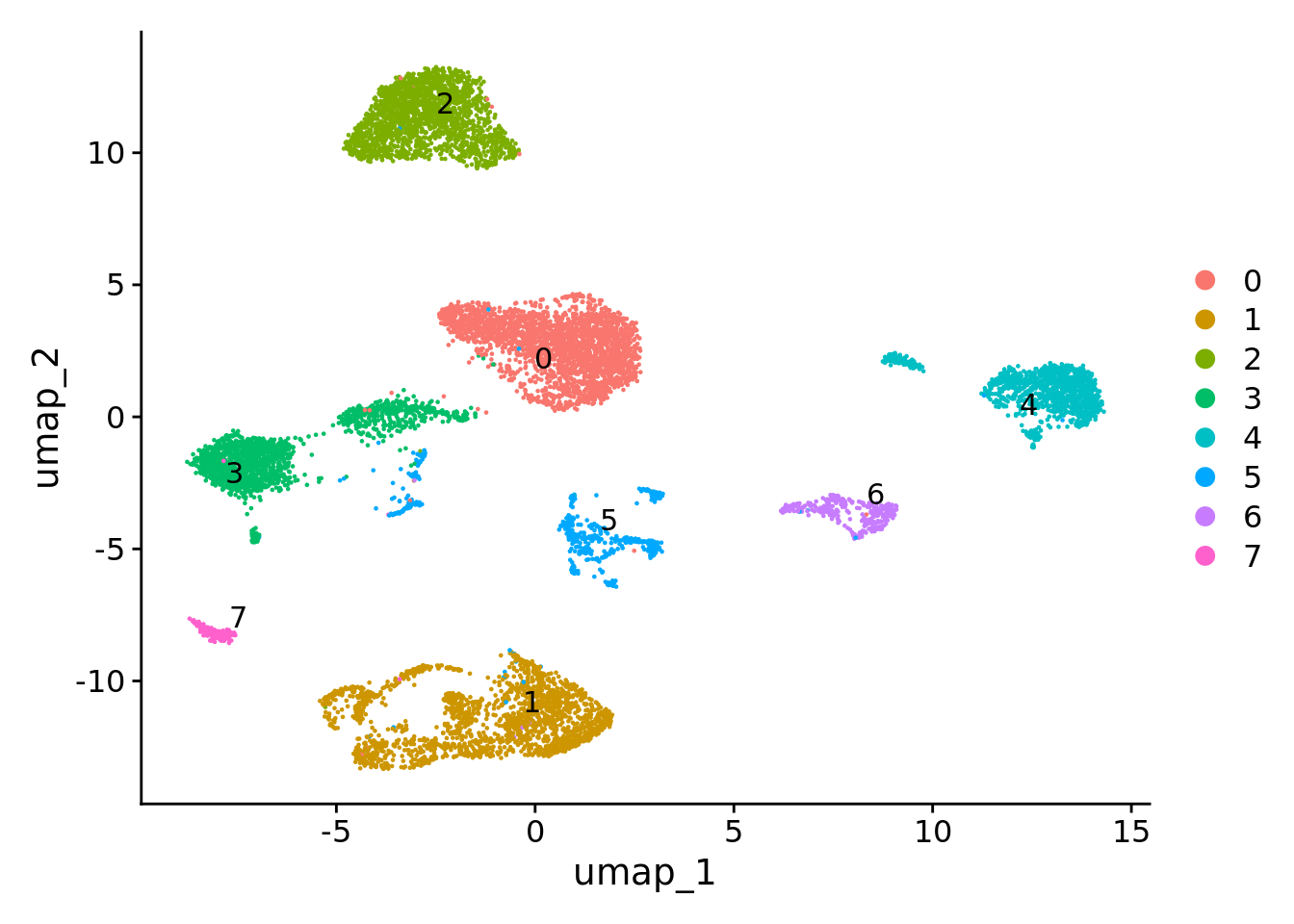
After removal of the doublets, the SCT normalization is repeated and the clustering is done with FindNeighbors and FindClusters.

Seurat <- SCTransform(Seurat, verbose = FALSE) #default variable features = 3000

Warning in theta.ml(Y, mu, sum(w), w, limit = control$maxit, trace =
control$trace > : iteration limit reached
Warning in theta.ml(Y, mu, sum(w), w, limit = control$maxit, trace =
control$trace > : iteration limit reached
Warning in theta.ml(Y, mu, sum(w), w, limit = control$maxit, trace =
control$trace > : iteration limit reached
Warning in theta.ml(Y, mu, sum(w), w, limit = control$maxit, trace =
control$trace > : iteration limit reached
Warning in theta.ml(Y, mu, sum(w), w, limit = control$maxit, trace =
control$trace > : iteration limit reached
Warning in theta.ml(Y, mu, sum(w), w, limit = control$maxit, trace =
control$trace > : iteration limit reached
Warning in theta.ml(Y, mu, sum(w), w, limit = control$maxit, trace =
control$trace > : iteration limit reached
Warning in theta.ml(Y, mu, sum(w), w, limit = control$maxit, trace =
control$trace > : iteration limit reached
Warning in theta.ml(Y, mu, sum(w), w, limit = control$maxit, trace =
control$trace > : iteration limit reached
Warning in theta.ml(Y, mu, sum(w), w, limit = control$maxit, trace =
control$trace > : iteration limit reached
Warning in theta.ml(Y, mu, sum(w), w, limit = control$maxit, trace =
control$trace > : iteration limit reached
Warning in theta.ml(Y, mu, sum(w), w, limit = control$maxit, trace =
control$trace > : iteration limit reached
Warning in theta.ml(Y, mu, sum(w), w, limit = control$maxit, trace =
control$trace > : iteration limit reached
Warning in theta.ml(Y, mu, sum(w), w, limit = control$maxit, trace =
control$trace > : iteration limit reached
Warning in theta.ml(Y, mu, sum(w), w, limit = control$maxit, trace =
control$trace > : iteration limit reached
Warning in theta.ml(Y, mu, sum(w), w, limit = control$maxit, trace =
control$trace > : iteration limit reached
Warning in theta.ml(Y, mu, sum(w), w, limit = control$maxit, trace =
control$trace > : iteration limit reached
Warning in theta.ml(Y, mu, sum(w), w, limit = control$maxit, trace =
control$trace > : iteration limit reached
Warning in theta.ml(Y, mu, sum(w), w, limit = control$maxit, trace =
control$trace > : iteration limit reached
Warning in theta.ml(Y, mu, sum(w), w, limit = control$maxit, trace =
control$trace > : iteration limit reached
Warning in theta.ml(Y, mu, sum(w), w, limit = control$maxit, trace =
control$trace > : iteration limit reached
Warning in theta.ml(Y, mu, sum(w), w, limit = control$maxit, trace =
control$trace > : iteration limit reached
Warning in theta.ml(Y, mu, sum(w), w, limit = control$maxit, trace =
control$trace > : iteration limit reached
Warning in theta.ml(Y, mu, sum(w), w, limit = control$maxit, trace =
control$trace > : iteration limit reached
Warning in theta.ml(Y, mu, sum(w), w, limit = control$maxit, trace =
control$trace > : iteration limit reached
Warning in theta.ml(Y, mu, sum(w), w, limit = control$maxit, trace =
control$trace > : iteration limit reached
Warning in theta.ml(Y, mu, sum(w), w, limit = control$maxit, trace =
control$trace > : iteration limit reached
Warning in theta.ml(Y, mu, sum(w), w, limit = control$maxit, trace =
control$trace > : iteration limit reached
Warning in theta.ml(Y, mu, sum(w), w, limit = control$maxit, trace =
control$trace > : iteration limit reached
Warning in theta.ml(Y, mu, sum(w), w, limit = control$maxit, trace =
control$trace > : iteration limit reached
Warning in theta.ml(Y, mu, sum(w), w, limit = control$maxit, trace =
control$trace > : iteration limit reached
Warning in theta.ml(Y, mu, sum(w), w, limit = control$maxit, trace =
control$trace > : iteration limit reached
Warning in theta.ml(Y, mu, sum(w), w, limit = control$maxit, trace =
control$trace > : iteration limit reached

Warning in sqrt(1/i): NaNs produced

Warning in theta.ml(Y, mu, sum(w), w, limit = control$maxit, trace =
control$trace > : iteration limit reached

Warning in sqrt(1/i): NaNs produced

Warning in theta.ml(Y, mu, sum(w), w, limit = control$maxit, trace =
control$trace > : iteration limit reached
Warning in theta.ml(Y, mu, sum(w), w, limit = control$maxit, trace =
control$trace > : iteration limit reached
Warning in theta.ml(Y, mu, sum(w), w, limit = control$maxit, trace =
control$trace > : iteration limit reached
Warning in theta.ml(Y, mu, sum(w), w, limit = control$maxit, trace =
control$trace > : iteration limit reached
Warning in theta.ml(Y, mu, sum(w), w, limit = control$maxit, trace =
control$trace > : iteration limit reached
Warning in theta.ml(Y, mu, sum(w), w, limit = control$maxit, trace =
control$trace > : iteration limit reached
Warning in theta.ml(Y, mu, sum(w), w, limit = control$maxit, trace =
control$trace > : iteration limit reached
Warning in theta.ml(Y, mu, sum(w), w, limit = control$maxit, trace =
control$trace > : iteration limit reached
Warning in theta.ml(Y, mu, sum(w), w, limit = control$maxit, trace =
control$trace > : iteration limit reached
Warning in theta.ml(Y, mu, sum(w), w, limit = control$maxit, trace =
control$trace > : iteration limit reached
Warning in theta.ml(Y, mu, sum(w), w, limit = control$maxit, trace =
control$trace > : iteration limit reached
Warning in theta.ml(Y, mu, sum(w), w, limit = control$maxit, trace =
control$trace > : iteration limit reached
Warning in theta.ml(Y, mu, sum(w), w, limit = control$maxit, trace =
control$trace > : iteration limit reached
Warning in theta.ml(Y, mu, sum(w), w, limit = control$maxit, trace =
control$trace > : iteration limit reached
Warning in theta.ml(Y, mu, sum(w), w, limit = control$maxit, trace =
control$trace > : iteration limit reached
Warning in theta.ml(Y, mu, sum(w), w, limit = control$maxit, trace =
control$trace > : iteration limit reached
Warning in theta.ml(Y, mu, sum(w), w, limit = control$maxit, trace =
control$trace > : iteration limit reached
Warning in theta.ml(Y, mu, sum(w), w, limit = control$maxit, trace =
control$trace > : iteration limit reached
Warning in theta.ml(Y, mu, sum(w), w, limit = control$maxit, trace =
control$trace > : iteration limit reached
Warning in theta.ml(Y, mu, sum(w), w, limit = control$maxit, trace =
control$trace > : iteration limit reached
Warning in theta.ml(Y, mu, sum(w), w, limit = control$maxit, trace =
control$trace > : iteration limit reached
Warning in theta.ml(Y, mu, sum(w), w, limit = control$maxit, trace =
control$trace > : iteration limit reached
Warning in theta.ml(Y, mu, sum(w), w, limit = control$maxit, trace =
control$trace > : iteration limit reached
Warning in theta.ml(Y, mu, sum(w), w, limit = control$maxit, trace =
control$trace > : iteration limit reached
Warning in theta.ml(Y, mu, sum(w), w, limit = control$maxit, trace =
control$trace > : iteration limit reached
Warning in theta.ml(Y, mu, sum(w), w, limit = control$maxit, trace =
control$trace > : iteration limit reached
Warning in theta.ml(Y, mu, sum(w), w, limit = control$maxit, trace =
control$trace > : iteration limit reached
Warning in theta.ml(Y, mu, sum(w), w, limit = control$maxit, trace =
control$trace > : iteration limit reached
Warning in theta.ml(Y, mu, sum(w), w, limit = control$maxit, trace =
control$trace > : iteration limit reached
Warning in theta.ml(Y, mu, sum(w), w, limit = control$maxit, trace =
control$trace > : iteration limit reached
Warning in theta.ml(Y, mu, sum(w), w, limit = control$maxit, trace =
control$trace > : iteration limit reached
Warning in theta.ml(Y, mu, sum(w), w, limit = control$maxit, trace =
control$trace > : iteration limit reached
Warning in theta.ml(Y, mu, sum(w), w, limit = control$maxit, trace =
control$trace > : iteration limit reached
Warning in theta.ml(Y, mu, sum(w), w, limit = control$maxit, trace =
control$trace > : iteration limit reached
Warning in theta.ml(Y, mu, sum(w), w, limit = control$maxit, trace =
control$trace > : iteration limit reached
Warning in theta.ml(Y, mu, sum(w), w, limit = control$maxit, trace =
control$trace > : iteration limit reached
Warning in theta.ml(Y, mu, sum(w), w, limit = control$maxit, trace =
control$trace > : iteration limit reached
Warning in theta.ml(Y, mu, sum(w), w, limit = control$maxit, trace =
control$trace > : iteration limit reached
Warning in theta.ml(Y, mu, sum(w), w, limit = control$maxit, trace =
control$trace > : iteration limit reached
Warning in theta.ml(Y, mu, sum(w), w, limit = control$maxit, trace =
control$trace > : iteration limit reached
Warning in theta.ml(Y, mu, sum(w), w, limit = control$maxit, trace =
control$trace > : iteration limit reached
Warning in theta.ml(Y, mu, sum(w), w, limit = control$maxit, trace =
control$trace > : iteration limit reached
Warning in theta.ml(Y, mu, sum(w), w, limit = control$maxit, trace =
control$trace > : iteration limit reached
Warning in theta.ml(Y, mu, sum(w), w, limit = control$maxit, trace =
control$trace > : iteration limit reached
Warning in theta.ml(Y, mu, sum(w), w, limit = control$maxit, trace =
control$trace > : iteration limit reached
Warning in theta.ml(Y, mu, sum(w), w, limit = control$maxit, trace =
control$trace > : iteration limit reached
Warning in theta.ml(Y, mu, sum(w), w, limit = control$maxit, trace =
control$trace > : iteration limit reached
Warning in theta.ml(Y, mu, sum(w), w, limit = control$maxit, trace =
control$trace > : iteration limit reached
Warning in theta.ml(Y, mu, sum(w), w, limit = control$maxit, trace =
control$trace > : iteration limit reached
Warning in theta.ml(Y, mu, sum(w), w, limit = control$maxit, trace =
control$trace > : iteration limit reached
Warning in theta.ml(Y, mu, sum(w), w, limit = control$maxit, trace =
control$trace > : iteration limit reached
Warning in theta.ml(Y, mu, sum(w), w, limit = control$maxit, trace =
control$trace > : iteration limit reached
Warning in theta.ml(Y, mu, sum(w), w, limit = control$maxit, trace =
control$trace > : iteration limit reached
Warning in theta.ml(Y, mu, sum(w), w, limit = control$maxit, trace =
control$trace > : iteration limit reached
Warning in theta.ml(Y, mu, sum(w), w, limit = control$maxit, trace =
control$trace > : iteration limit reached
Warning in theta.ml(Y, mu, sum(w), w, limit = control$maxit, trace =
control$trace > : iteration limit reached
Warning in theta.ml(Y, mu, sum(w), w, limit = control$maxit, trace =
control$trace > : iteration limit reached
Warning in theta.ml(Y, mu, sum(w), w, limit = control$maxit, trace =
control$trace > : iteration limit reached
Warning in theta.ml(Y, mu, sum(w), w, limit = control$maxit, trace =
control$trace > : iteration limit reached
Warning in theta.ml(Y, mu, sum(w), w, limit = control$maxit, trace =
control$trace > : iteration limit reached
Warning in theta.ml(Y, mu, sum(w), w, limit = control$maxit, trace =
control$trace > : iteration limit reached
Warning in theta.ml(Y, mu, sum(w), w, limit = control$maxit, trace =
control$trace > : iteration limit reached
Warning in theta.ml(Y, mu, sum(w), w, limit = control$maxit, trace =
control$trace > : iteration limit reached
Warning in theta.ml(Y, mu, sum(w), w, limit = control$maxit, trace =
control$trace > : iteration limit reached
Warning in theta.ml(Y, mu, sum(w), w, limit = control$maxit, trace =
control$trace > : iteration limit reached
Warning in theta.ml(Y, mu, sum(w), w, limit = control$maxit, trace =
control$trace > : iteration limit reached
Warning in theta.ml(Y, mu, sum(w), w, limit = control$maxit, trace =
control$trace > : iteration limit reached
Warning in theta.ml(Y, mu, sum(w), w, limit = control$maxit, trace =
control$trace > : iteration limit reached
Warning in theta.ml(Y, mu, sum(w), w, limit = control$maxit, trace =
control$trace > : iteration limit reached
Warning in theta.ml(Y, mu, sum(w), w, limit = control$maxit, trace =
control$trace > : iteration limit reached
Warning in theta.ml(Y, mu, sum(w), w, limit = control$maxit, trace =
control$trace > : iteration limit reached
Warning in theta.ml(Y, mu, sum(w), w, limit = control$maxit, trace =
control$trace > : iteration limit reached
Warning in theta.ml(Y, mu, sum(w), w, limit = control$maxit, trace =
control$trace > : iteration limit reached
Warning in theta.ml(Y, mu, sum(w), w, limit = control$maxit, trace =
control$trace > : iteration limit reached
Warning in theta.ml(Y, mu, sum(w), w, limit = control$maxit, trace =
control$trace > : iteration limit reached

Warning in sqrt(1/i): NaNs produced

Warning in theta.ml(Y, mu, sum(w), w, limit = control$maxit, trace =
control$trace > : iteration limit reached

Warning in sqrt(1/i): NaNs produced

Warning in theta.ml(Y, mu, sum(w), w, limit = control$maxit, trace =
control$trace > : iteration limit reached
Warning in theta.ml(Y, mu, sum(w), w, limit = control$maxit, trace =
control$trace > : iteration limit reached
Warning in theta.ml(Y, mu, sum(w), w, limit = control$maxit, trace =
control$trace > : iteration limit reached
Warning in theta.ml(Y, mu, sum(w), w, limit = control$maxit, trace =
control$trace > : iteration limit reached
Warning in theta.ml(Y, mu, sum(w), w, limit = control$maxit, trace =
control$trace > : iteration limit reached
Warning in theta.ml(Y, mu, sum(w), w, limit = control$maxit, trace =
control$trace > : iteration limit reached
Warning in theta.ml(Y, mu, sum(w), w, limit = control$maxit, trace =
control$trace > : iteration limit reached
Warning in theta.ml(Y, mu, sum(w), w, limit = control$maxit, trace =
control$trace > : iteration limit reached
Warning in theta.ml(Y, mu, sum(w), w, limit = control$maxit, trace =
control$trace > : iteration limit reached
Warning in theta.ml(Y, mu, sum(w), w, limit = control$maxit, trace =
control$trace > : iteration limit reached
Warning in theta.ml(Y, mu, sum(w), w, limit = control$maxit, trace =
control$trace > : iteration limit reached
Warning in theta.ml(Y, mu, sum(w), w, limit = control$maxit, trace =
control$trace > : iteration limit reached
Warning in theta.ml(Y, mu, sum(w), w, limit = control$maxit, trace =
control$trace > : iteration limit reached
Warning in theta.ml(Y, mu, sum(w), w, limit = control$maxit, trace =
control$trace > : iteration limit reached
Warning in theta.ml(Y, mu, sum(w), w, limit = control$maxit, trace =
control$trace > : iteration limit reached
Warning in theta.ml(Y, mu, sum(w), w, limit = control$maxit, trace =
control$trace > : iteration limit reached
Warning in theta.ml(Y, mu, sum(w), w, limit = control$maxit, trace =
control$trace > : iteration limit reached
Warning in theta.ml(Y, mu, sum(w), w, limit = control$maxit, trace =
control$trace > : iteration limit reached
Warning in theta.ml(Y, mu, sum(w), w, limit = control$maxit, trace =
control$trace > : iteration limit reached
Warning in theta.ml(Y, mu, sum(w), w, limit = control$maxit, trace =
control$trace > : iteration limit reached
Warning in theta.ml(Y, mu, sum(w), w, limit = control$maxit, trace =
control$trace > : iteration limit reached
Warning in theta.ml(Y, mu, sum(w), w, limit = control$maxit, trace =
control$trace > : iteration limit reached
Warning in theta.ml(Y, mu, sum(w), w, limit = control$maxit, trace =
control$trace > : iteration limit reached
Warning in theta.ml(Y, mu, sum(w), w, limit = control$maxit, trace =
control$trace > : iteration limit reached
Warning in theta.ml(Y, mu, sum(w), w, limit = control$maxit, trace =
control$trace > : iteration limit reached
Warning in theta.ml(Y, mu, sum(w), w, limit = control$maxit, trace =
control$trace > : iteration limit reached
Warning in theta.ml(Y, mu, sum(w), w, limit = control$maxit, trace =
control$trace > : iteration limit reached
Warning in theta.ml(Y, mu, sum(w), w, limit = control$maxit, trace =
control$trace > : iteration limit reached
Warning in theta.ml(Y, mu, sum(w), w, limit = control$maxit, trace =
control$trace > : iteration limit reached
Warning in theta.ml(Y, mu, sum(w), w, limit = control$maxit, trace =
control$trace > : iteration limit reached
Warning in theta.ml(Y, mu, sum(w), w, limit = control$maxit, trace =
control$trace > : iteration limit reached
Warning in theta.ml(Y, mu, sum(w), w, limit = control$maxit, trace =
control$trace > : iteration limit reached
Warning in theta.ml(Y, mu, sum(w), w, limit = control$maxit, trace =
control$trace > : iteration limit reached
Warning in theta.ml(Y, mu, sum(w), w, limit = control$maxit, trace =
control$trace > : iteration limit reached
Warning in theta.ml(Y, mu, sum(w), w, limit = control$maxit, trace =
control$trace > : iteration limit reached
Warning in theta.ml(Y, mu, sum(w), w, limit = control$maxit, trace =
control$trace > : iteration limit reached
Warning in theta.ml(Y, mu, sum(w), w, limit = control$maxit, trace =
control$trace > : iteration limit reached
Warning in theta.ml(Y, mu, sum(w), w, limit = control$maxit, trace =
control$trace > : iteration limit reached
Warning in theta.ml(Y, mu, sum(w), w, limit = control$maxit, trace =
control$trace > : iteration limit reached
Warning in theta.ml(Y, mu, sum(w), w, limit = control$maxit, trace =
control$trace > : iteration limit reached
Warning in theta.ml(Y, mu, sum(w), w, limit = control$maxit, trace =
control$trace > : iteration limit reached
Warning in theta.ml(Y, mu, sum(w), w, limit = control$maxit, trace =
control$trace > : iteration limit reached
Warning in theta.ml(Y, mu, sum(w), w, limit = control$maxit, trace =
control$trace > : iteration limit reached
Warning in theta.ml(Y, mu, sum(w), w, limit = control$maxit, trace =
control$trace > : iteration limit reached
Warning in theta.ml(Y, mu, sum(w), w, limit = control$maxit, trace =
control$trace > : iteration limit reached
Warning in theta.ml(Y, mu, sum(w), w, limit = control$maxit, trace =
control$trace > : iteration limit reached
Warning in theta.ml(Y, mu, sum(w), w, limit = control$maxit, trace =
control$trace > : iteration limit reached
Warning in theta.ml(Y, mu, sum(w), w, limit = control$maxit, trace =
control$trace > : iteration limit reached
Warning in theta.ml(Y, mu, sum(w), w, limit = control$maxit, trace =
control$trace > : iteration limit reached
Warning in theta.ml(Y, mu, sum(w), w, limit = control$maxit, trace =
control$trace > : iteration limit reached
Warning in theta.ml(Y, mu, sum(w), w, limit = control$maxit, trace =
control$trace > : iteration limit reached
Warning in theta.ml(Y, mu, sum(w), w, limit = control$maxit, trace =
control$trace > : iteration limit reached
Warning in theta.ml(Y, mu, sum(w), w, limit = control$maxit, trace =
control$trace > : iteration limit reached
Warning in theta.ml(Y, mu, sum(w), w, limit = control$maxit, trace =
control$trace > : iteration limit reached
Warning in theta.ml(Y, mu, sum(w), w, limit = control$maxit, trace =
control$trace > : iteration limit reached
Warning in theta.ml(Y, mu, sum(w), w, limit = control$maxit, trace =
control$trace > : iteration limit reached
Warning in theta.ml(Y, mu, sum(w), w, limit = control$maxit, trace =
control$trace > : iteration limit reached
Warning in theta.ml(Y, mu, sum(w), w, limit = control$maxit, trace =
control$trace > : iteration limit reached
Warning in theta.ml(Y, mu, sum(w), w, limit = control$maxit, trace =
control$trace > : iteration limit reached
Warning in theta.ml(Y, mu, sum(w), w, limit = control$maxit, trace =
control$trace > : iteration limit reached
Warning in theta.ml(Y, mu, sum(w), w, limit = control$maxit, trace =
control$trace > : iteration limit reached
Warning in theta.ml(Y, mu, sum(w), w, limit = control$maxit, trace =
control$trace > : iteration limit reached
Warning in theta.ml(Y, mu, sum(w), w, limit = control$maxit, trace =
control$trace > : iteration limit reached
Warning in theta.ml(Y, mu, sum(w), w, limit = control$maxit, trace =
control$trace > : iteration limit reached
Warning in theta.ml(Y, mu, sum(w), w, limit = control$maxit, trace =
control$trace > : iteration limit reached
Warning in theta.ml(Y, mu, sum(w), w, limit = control$maxit, trace =
control$trace > : iteration limit reached
Warning in theta.ml(Y, mu, sum(w), w, limit = control$maxit, trace =
control$trace > : iteration limit reached
Warning in theta.ml(Y, mu, sum(w), w, limit = control$maxit, trace =
control$trace > : iteration limit reached
Warning in theta.ml(Y, mu, sum(w), w, limit = control$maxit, trace =
control$trace > : iteration limit reached
Warning in theta.ml(Y, mu, sum(w), w, limit = control$maxit, trace =
control$trace > : iteration limit reached
Warning in theta.ml(Y, mu, sum(w), w, limit = control$maxit, trace =
control$trace > : iteration limit reached
Warning in theta.ml(Y, mu, sum(w), w, limit = control$maxit, trace =
control$trace > : iteration limit reached
Warning in theta.ml(Y, mu, sum(w), w, limit = control$maxit, trace =
control$trace > : iteration limit reached
Warning in theta.ml(Y, mu, sum(w), w, limit = control$maxit, trace =
control$trace > : iteration limit reached
Warning in theta.ml(Y, mu, sum(w), w, limit = control$maxit, trace =
control$trace > : iteration limit reached
Warning in theta.ml(Y, mu, sum(w), w, limit = control$maxit, trace =
control$trace > : iteration limit reached
Warning in theta.ml(Y, mu, sum(w), w, limit = control$maxit, trace =
control$trace > : iteration limit reached
Warning in theta.ml(Y, mu, sum(w), w, limit = control$maxit, trace =
control$trace > : iteration limit reached
Warning in theta.ml(Y, mu, sum(w), w, limit = control$maxit, trace =
control$trace > : iteration limit reached
Warning in theta.ml(Y, mu, sum(w), w, limit = control$maxit, trace =
control$trace > : iteration limit reached

Warning: Different cells and/or features from existing assay SCT

Seurat <- RunPCA(Seurat, verbose = FALSE)
Seurat <- RunUMAP(Seurat, reduction = "pca",dims = 1:30, verbose = FALSE)
Seurat <- FindNeighbors(Seurat, reduction = "pca",dims = 1:30)
Seurat <- FindClusters(Seurat,resolution = 0.05)

Modularity Optimizer version 1.3.0 by Ludo Waltman and Nees Jan van Eck

Number of nodes: 10582
Number of edges: 420910

Running Louvain algorithm...
Maximum modularity in 10 random starts: 0.9890
Number of communities: 8
Elapsed time: 1 seconds

Eight clusters were originated for a clustering resolution of 0.05.

DimPlot(Seurat, reduction = "umap", label = TRUE, repel = TRUE)

Annotated by Sample_ID.

DimPlot(Seurat, reduction = "umap", label = FALSE, repel = TRUE, group.by = "Sample_ID")

Calculate gene markers for each cluster

Use FindAllMarkers to calculate the markers for each cluster.

Seurat.markers <- FindAllMarkers(Seurat, only.pos = TRUE, min.pct = 0.1, logfc.threshold = 0.25)

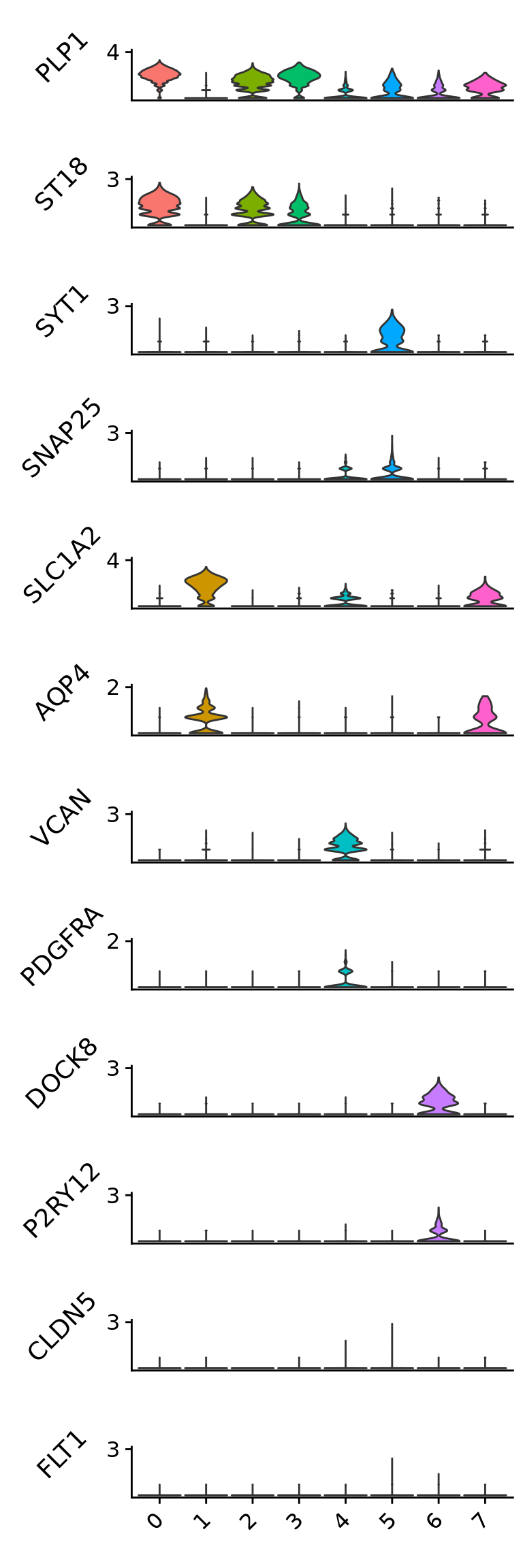
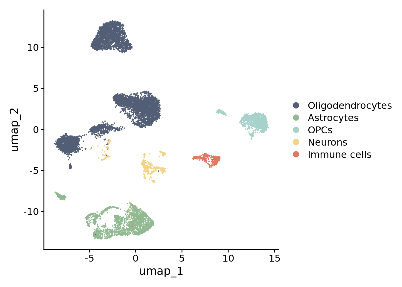
Upload the list of canonical cell-type markers collected from the literature that is located at the “Support data” folder of this repository. Check for canonical markers within Seurat.markers.

known_markers <- merge(Seurat.markers, Brain_cell_markers, by="gene")

Check the expression of some canonical markers to guide cluster annotation. Script for the stacked violin plot function:

## remove the x-axis text and tick
## plot.margin to adjust the white space between each plot.
## ... pass any arguments to VlnPlot in Seurat
modify_vlnplot<- function(obj,
feature,
pt.size = 0,
plot.margin = unit(c(-0.75, 0, -0.75, 0), "cm"),
...) {
p<- VlnPlot(obj, features = feature, pt.size = pt.size #,cols = UMAP_colors
, ... ) +
xlab("") + ylab(feature) + ggtitle("") +
theme(legend.position = "none",
axis.text.x = element_blank(),
axis.ticks.x = element_blank(),
axis.title.y = element_text(size = rel(1), angle = 45),
axis.text.y = element_text(size = rel(1)),
plot.margin = plot.margin )
return(p)
}
## extract the max value of the y axis
extract_max<- function(p){
ymax<- max(ggplot_build(p)$layout$panel_scales_y[[1]]$range$range)
return(ceiling(ymax))
}
## main function
StackedVlnPlot<- function(obj, features,
pt.size = 0,
plot.margin = unit(c(-0.75, 0, -0.75, 0), "cm"),
...) {
plot_list<- purrr::map(features, function(x) modify_vlnplot(obj = obj,feature = x, ...))
# Add back x-axis title to bottom plot. patchwork is going to support this?
plot_list[[length(plot_list)]]<- plot_list[[length(plot_list)]] +
theme(axis.text.x=element_text(angle = 45, hjust = 1), axis.ticks.x = element_line())
# change the y-axis tick to only max value
ymaxs<- purrr::map_dbl(plot_list, extract_max)
plot_list<- purrr::map2(plot_list, ymaxs, function(x,y) x +
scale_y_continuous(breaks = c(y)) +
expand_limits(y = y))
p<- patchwork::wrap_plots(plotlist = plot_list, ncol = 1)
return(p)
}

Stacked violin plots

markers<- c("PLP1","ST18",  #OLIGO
"SYT1", "SNAP25",           #NEURONS
"SLC1A2", "AQP4",           #ASTROCYTES
"VCAN", "PDGFRA",           #OPCS
"DOCK8", "P2RY12",          #IMMUNE CELLS
"CLDN5", "FLT1")            #ENDOT

StackedVlnPlot(obj = Seurat, features = markers)

Assign new cluster ids for cell types based on marker expression

Make this assessment based on the previous information.

new.cluster.ids <- c("Oligodendrocytes", "Astrocytes","Oligodendrocytes","Oligodendrocytes","OPCs","Neurons","Immune cells","Astrocytes")
names(new.cluster.ids) <- levels(Seurat)
Seurat <- RenameIdents(Seurat, new.cluster.ids)

Feature plot with the Module score of the expression of microglia/immune cell markers.

DefaultAssay(Seurat) <- "SCT"
Immune_genes <-c( "P2RY12","DOCK8","CD74","CX3CR1","C1QB","C3","AIF1","HLA-DRA")
Seurat <- AddModuleScore(Seurat,features =list(Immune_genes),name='Immune_genes')
FeaturePlot(Seurat, features = "Immune_genes1",cols = c("#F1EEE9","#DF7861"))

Color the UMAP plot by cell-type.

UMAP_colors<-c("#525E75", #Oligodendrocytes
"#92BA92",                #Astrocytes
"#A7D2CB",                #OPCs
"#F2D388",                #Neurons
"#DF7861"                 #Immune cells
)

DimPlot(Seurat, reduction = "umap", label = FALSE, repel = F ,cols = UMAP_colors)

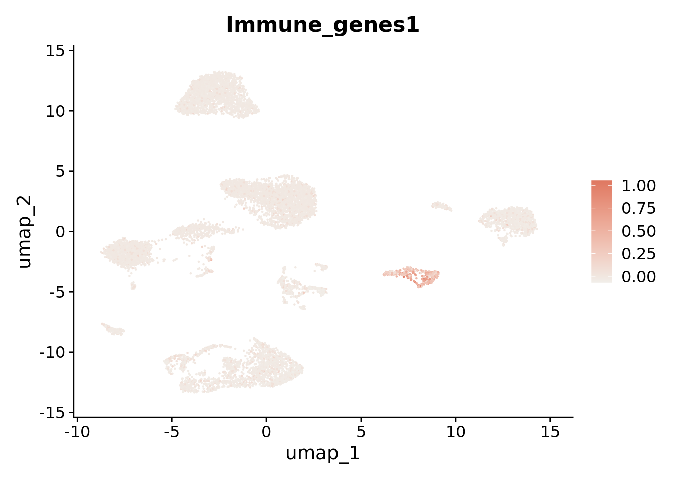
Subset the immune cell cluster from the Seurat object

The nuclei annotated as belonging to immune cells are singled-out in an individual Seurat object, consisting of 340 nuclei, to be later integrated with the other datasets to form the
Human Microglia Atlas (HuMicA).

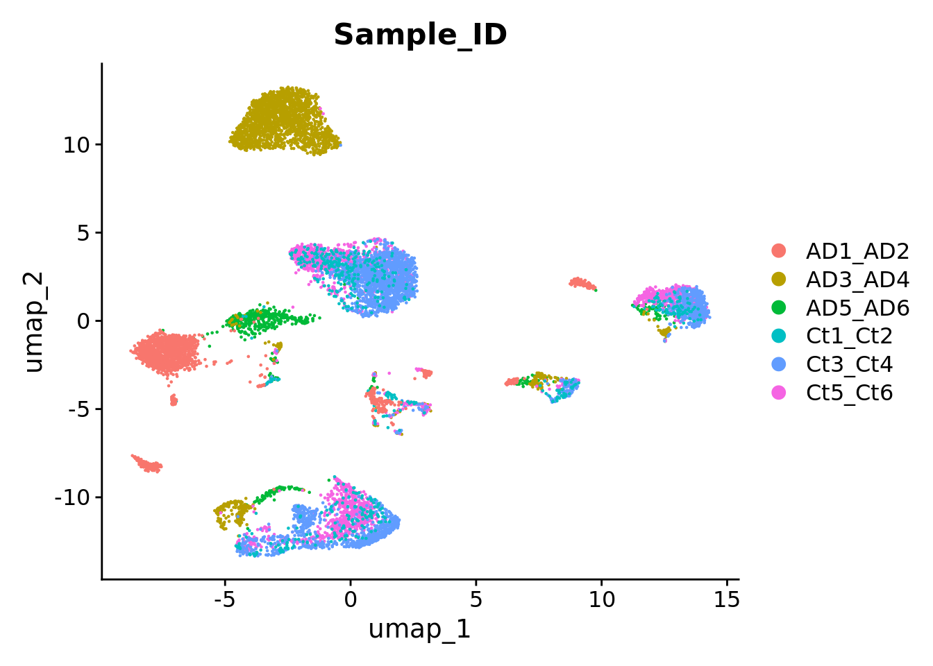
Immune_Seurat<- Seurat[,Seurat@active.ident=="Immune cells"]

Check for outlier samples

The last step consist on verifying if any of the samples within the filtered object shows an unbalanced number of nuclei. In this case, all samples have an approximate number of nuclei. Therefore, all were included in the final integration.

md <- Immune_Seurat@meta.data %>% as.data.table
Cell_number_subject <- md[, .N, by = c("Sample_ID")]
Cell_number_subject

   Sample_ID     N
      <char> <int>
1:   AD5_AD6    29
2:   AD3_AD4    84
3:   Ct5_Ct6    55
4:   Ct3_Ct4    83
5:   Ct1_Ct2    39
6:   AD1_AD2    45